This final chapter is a brief survey of various methods that go beyond standard linear regression. In particular, we we look at generalized linear models, Neural Networks, and non-parametric regression.
4.1 Generalized Linear Models
A generalized linear model (GLM) extends the usual linear model to cases where the errors \(\varepsilon\) have proposed distributions that are very different than the normal distribution. In this case, we assume that \(\varepsilon\) comes from an exponential family, and the form of the model is \[
g\left( \mathrm{E}y \right) =
\beta_0 + \beta_1x_1 +\ldots+ \beta_px_p.
\] Here, \(g(\cdot)\) is referred to as the link function. As these are still parametric models, the parameters \(\beta_0,\ldots,\beta_p\) are often solved for via maximum likelihood. These models can be fit in R via the glm() function. While such models can be studied in full generality, for this course, we will only consider two specific GLMs: the logistic regression and the Poisson regression.
4.1.1 Logistic Regression
One of the most useful GLMs is the logistic regression. This is applied in the case of a binary response–i.e when \(y\in\{0,1\}\). This could, for example, be used for diagnosis of a disease where \(x_1,\ldots,x_p\) are predictors and \(y\) corresponds to the presence or absence of the disease.
The usual setup is to treat the observed responses \(y_i\in\{0,1\}\) as \(\mathrm{Bernoulli}\left(\pi_i\right)\) random variables, which is \[
\mathrm{P}\left(y_i=1\right)=\pi_i~\text{ and }~\mathrm{P}\left(y_i=0\right)=1-\pi_i.
\] This implies that the mean is \(\mathrm{E}{y_i}=\pi_i\) and the variance is \(\mathrm{Var}\left(y_i\right) = \pi_i(1-\pi_i)\). Hence, the variance is a function of the mean, which violates the assumption of constant variance in the Gauss-Markov theorem.
The goal is then to model \(\mathrm{E}{y_i}=\pi_i\) as a function of \({x}^\mathrm{T}_i\beta\). While different link functions are possible—see, for example, probit regression—the standard link function chosen is the logistic response function, sometimes referred to as the logit function, which is \[
\mathrm{E}y_i = \pi_i =
\frac{\exp({x}^\mathrm{T}_i\beta)}{1+\exp({x}^\mathrm{T}_i\beta)}
\] and results in an S-shaped curve. Rearranging the equation results in \[
\log\left( \frac{\pi_i}{1-\pi_i} \right)
= {x}^\mathrm{T}_i\beta = \beta_0 + \beta_1x_{i,1}+\ldots+\beta_px_{i,p}
\] where the ratio \(\pi_i/(1-\pi_i)\) is the odds ratio or simply the odds. Furthermore, the entire response \(\log\left( {\pi_i}/({1-\pi_i}) \right)\) is often referred to as the log odds.
The estimator \(\hat{\beta}\) can be computed numerically via maximum likelihood as we assume the underlying distribution of the data. Hence, we also get fitted values of the form \[
\hat{y}_i = \hat{\pi}_i =
\frac{\exp{({x}^\mathrm{T}_i\hat{\beta}})}{1+\exp{({x}^\mathrm{T}_i\hat{\beta}})}.
\] However, as noted already, the variance is not constant. Hence, for residuals of the form \(y_i-\hat{\pi}_i\) to be useful, we will need to normalize them. The Pearson residual for the logistic regression is \[
r_i = \frac{y_i - \hat{\pi}_i}{\sqrt{\hat{\pi}_i(1-\hat{\pi}_i)}}.
\]
4.1.1.1 Binomial responses
In some cases, multiple observations can be made for each value of predictors \(x\). For example, \(x_i\in\mathbb{R}^+\) could correspond to a dosage of medication and \(y_i\in\{0,1,\ldots,m_i\}\) could correspond to the number of the \(m_i\) subjects treated with dosage \(x_i\) that are cured of whatever ailment the medication was supposed to treat.
In this setting, we can treat the observed values \(\pi_i = y_i/m_i\). Often when fitting a logistic regression model to binomial data, the data points are weighted with respect to the number of observations \(m_i\) at each regressor \(x_i\). That is, if \(m_1\) is very large and \(m_2\) is small, then the estimation of \(\pi_1 = y_1/m_1\) is more accurate–i.e. lower variance–than \(\pi_2 =y_2/m_2\).
4.1.1.2 Testing model fit
Estimation of the parameters \(\beta\) is achieved by finding the maximum likelihood estimator. The log likelihood in the logistic regression with Bernoulli data is \[\begin{align*}
\log L(\beta)
&= \log \prod_{i=1}^n \pi_i^{y_i}(1-\pi_i)^{1-y_i}\\
&= \sum_{i=1}^n\left[
y_i\log\pi_i + (1-y_i)\log(1-\pi_i)
\right]\\
&= \sum_{i=1}^n\left[
y_i\log\left(\frac{\pi_i}{1-\pi_i}\right) + \log(1-\pi_i)
\right]\\
&= \sum_{i=1}^n\left[
y_i{x}^\mathrm{T}_i\beta - \log(1+\mathrm{e}^{{x}^\mathrm{T}_i\beta})
\right].
\end{align*}\] The MLE \(\hat{\beta}\) is solved for numerically.
Beyond finding the MLEs, the log likelihood is also used to test for the goodness-of-fit of the regression model. This comes from a result known as Wilks’ theorem.
4.1.2 Wilks’ Theorem
For two statistical models with parameter spaces \(\Theta_0\) and \(\Theta_1\) such that \(\Theta_0\subset\Theta_1\)—i.e. the models are nested—and likelihoods \(L_0(\theta)\) and \(L_1(\theta)\), then -2 times the log likelihood ratio has an asymptotic chi-squared distribution with degrees of freedom equal to the difference in the dimensionality of the parameter spaces. That is, \[
-2\log(LR) =
-2\log\left(
\frac{
\sup_{\theta\in\Theta_0}L_0(\theta)
}{
\sup_{\theta\in\Theta_1}L_1(\theta)
}
\right) \xrightarrow{\text{d}} \chi^2\left(\lvert\Theta_1\rvert-\lvert\Theta_0\rvert\right).
\]
In the case of logistic regression, we can use this result to construct an analogue to the F-test when the errors have a normal distribution. That is, we can compute the likelihood of the constant model \[
\log\left(\frac{\pi_i}{1-\pi_i}\right) = \beta_0
\tag{4.1}\] and the likelihood of the full model \[
\log\left(\frac{\pi_i}{1-\pi_i}\right) =
\beta_0 + \beta_1x_1 + \ldots + \beta_px_p.
\tag{4.2}\] and claim from Wilks’ theorem that \(-2\log(LR)\) is approximately distributed \(\chi^2\left(p\right)\) assuming the sample size is large enough.
In R, the glm() function does not return a p-value as the lm() function does for the F test. Instead, it provides two values, the null and residual deviances, which are respectively \[\begin{align*}
\text{null deviance}
&= -2 \log\left(
\frac{L(\text{null model})}{L(\text{saturated model})}
\right), \text{ and}\\
\text{residual deviance}
&= -2 \log\left(
\frac{L(\text{full model})}{L(\text{saturated model})}
\right).
\end{align*}\] Here, the null model is from Equation 4.1 and the full model is from Equation 4.2. The saturated model is the extreme model with \(p=n\) parameters, which perfectly models the data. It is, in some sense, the largest possible model used as a baseline.
In practice, the deviances can be thought of like the residual sum of squares from the ordinary linear regression setting. If the decrease is significant, then the regressors have predictive power over the response. Furthermore, \[
(\text{null deviance})-(\text{residual deviance}) =
-2 \log\left(
\frac{L(\text{null model})}{L(\text{full model})}
\right),
\] which has an asymptotic \(\chi^2\left(p\right)\) distribution. Such a goodness of fit test can be run in R using anova( model, test="LRT" ). Note that there are other goodness-of-fit tests possible for such models.
4.1.2.1 Logistic Regression: An Example
A sample of size \(n=21\) was randomly generated with \(x_i\in[-1,1]\) and \(y_i\) such that \[
y_i\sim\mathrm{Bernoulli}\left(
\frac{\mathrm{e}^{2x_i}}{1+\mathrm{e}^{2x_i}}
\right).
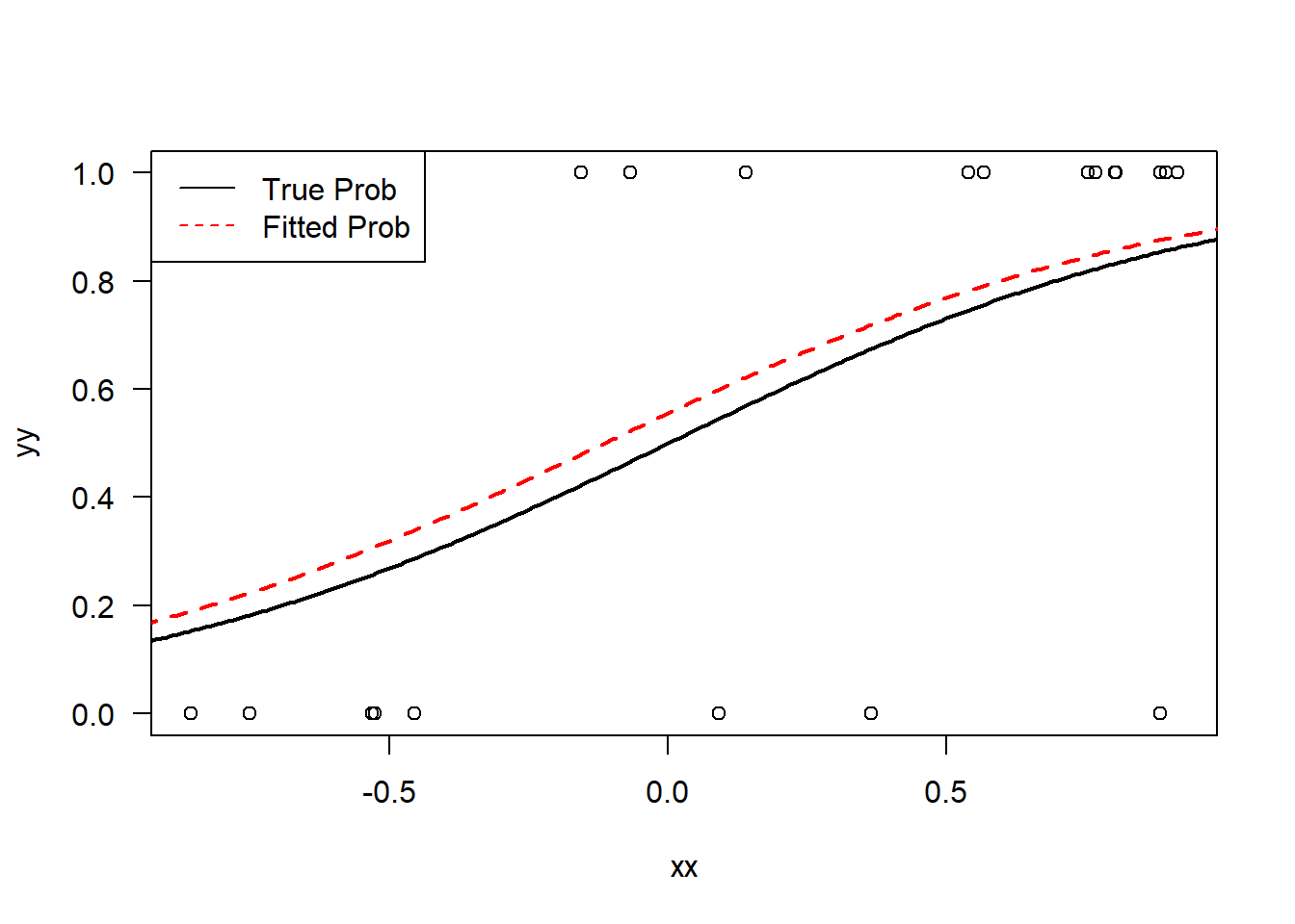
\] A logistic regression was fit to the data in R using the glm() function with the family=binomial(logit) argument to specify that the distribution is Bernoulli–i.e. binomial with \(n=1\)–and that we want a logistic link function.
The result from summary() is the model \[
\log\left( \frac{\pi}{1-\pi} \right) =
0.224 + 1.959 x
\] with a p-value of \(0.029\) for \(\hat{\beta_1}=1.959\). A plot of the true and predicted curves is displayed below.
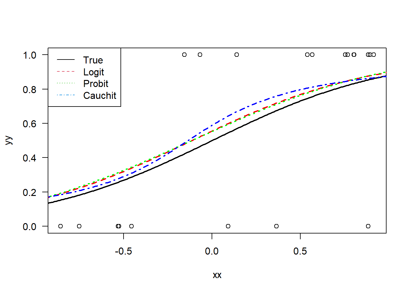
With the same data, we also fit a probit and cauchit model. These replace the logit link function with the CDF of the normal distribution (probit) or the CDF of the Cauchy distribution (cauchit). This latter case is the \(\arctan()\) function.
We could consider the alternative case were \[
y_i\sim\mathrm{Binomial}\left(m_i,
\frac{\mathrm{e}^{2x_i}}{1+\mathrm{e}^{2x_i}}
\right)
\] for some \(m_i\in\mathbb{Z}^+\), which is \(m_i\) Bernoulli observations at each \(x_i\). In this case, we have a much larger dataset.
# Generate Some Dataset.seed(378)nn <-21xx <-runif(nn,-1,1)pp <-exp( 2*xx )/( 1+exp( 2*xx ) )yy <-rbinom( nn, 1, prob=pp )## plot dataplot( xx, yy, las=1)## Fit a logistic Regressionmd.logit <-glm( yy~xx, family =binomial(link="logit"))summary(md.logit)
Call:
glm(formula = yy ~ xx, family = binomial(link = "logit"))

Coefficients:
            Estimate Std. Error z value Pr(>|z|)
(Intercept)   0.2244     0.5345   0.420   0.6746
xx            1.9589     0.8941   2.191   0.0285 *
---
Signif. codes:  0 '***' 0.001 '**' 0.01 '*' 0.05 '.' 0.1 ' ' 1

(Dispersion parameter for binomial family taken to be 1)

    Null deviance: 27.910  on 20  degrees of freedom
Residual deviance: 21.779  on 19  degrees of freedom
AIC: 25.779

Number of Fisher Scoring iterations: 4
## Do a probit and a cauchit model as wellmd.pro <-glm( yy~xx, family =binomial(link="probit"))md.cau <-glm( yy~xx, family =binomial(link="cauchit"))plot( xx, yy, las=1)lines( tt, exp( 2*tt )/( 1+exp( 2*tt ) ),col ='black', lwd=2)lines( tt, prd.logit, lwd=2,col ='red', lty=2)prd.pro =predict( md.pro, data.frame(xx=tt),type ="response")prd.cau =predict( md.cau, data.frame(xx=tt),type ="response")lines( tt, prd.pro, lwd=2,col ='green', lty=3)lines( tt, prd.cau, lwd=2,col ='blue', lty=4)legend("topleft",legend =c("True","Logit","Probit","Cauchit"),col=1:4,lty=1:4)
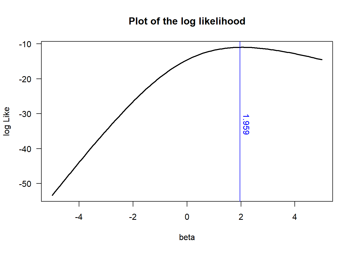
While we cannot solve for a closed form solution, we can numerically calculate the likelihood function for different choices of \(\beta\). This is done in the below R code with a blue line indicating the MLE found in the previous chunk of code.
# some candidate betasbet =seq(-5,5,0.1)like =0*bet;for( ii in1:length(bet) ) like[ii] =sum( yy*xx*bet[ii] -log( 1+exp(xx*bet[ii]) ) )plot( bet,like,type='l',las=1,xlab="beta",ylab="log Like",main="Plot of the log likelihood",lwd=2)abline( v =1.959, col='blue' )text( x=2,y=-30,labels="1.959",pos=4,srt=270, col='blue' )
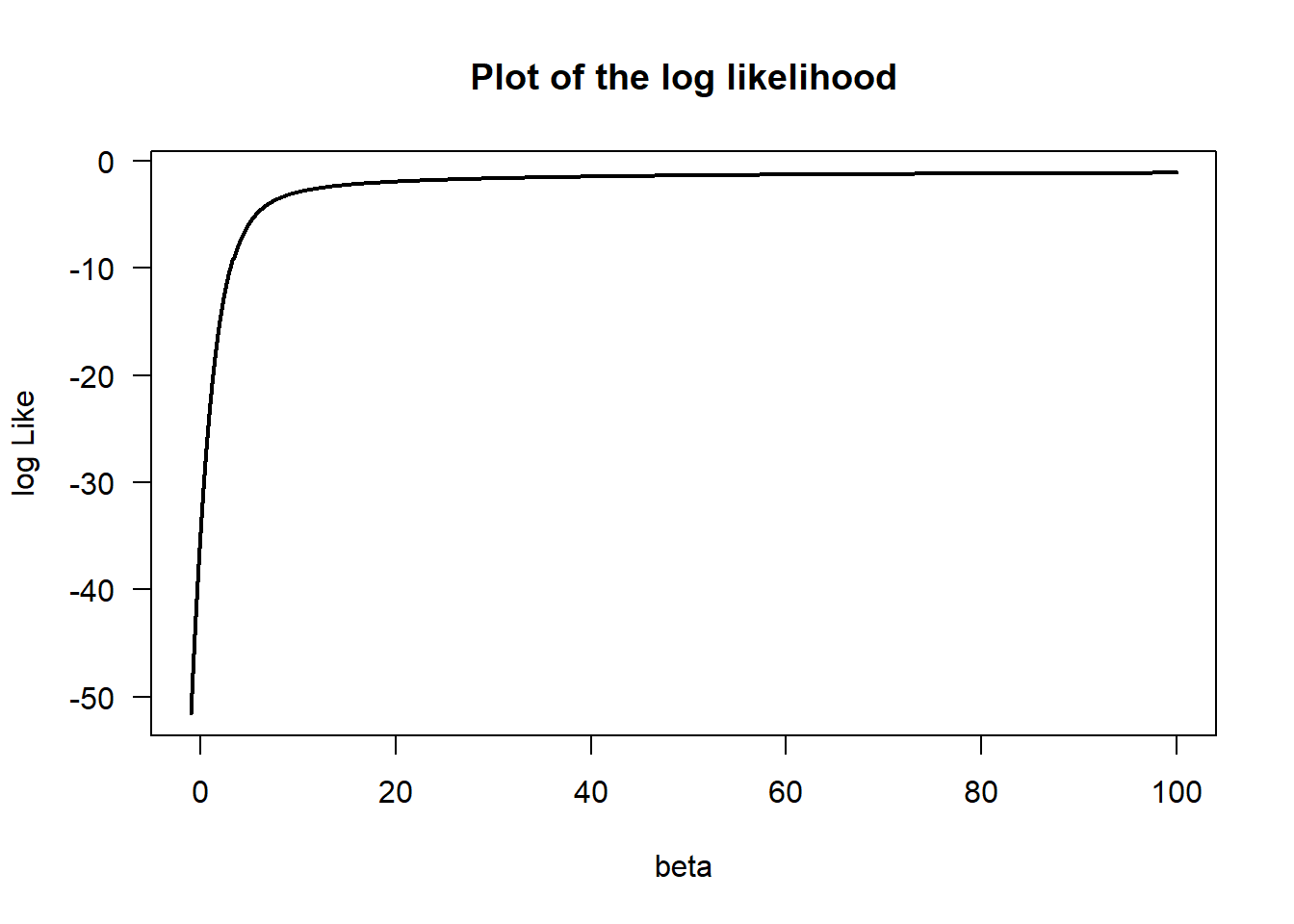
Another interesting property to note is that in logistic regression is that it does not work correctly if the data is perfectly separated by a hyperplane. This is in contrast to methods like support vector machines. The reason for logisitic regression’s failure is the fact that the MLE becomes maximized at infinity. We have another similar chunk of code below to plot this likelihood function.
xx =runif(50,-1,1)yy = xx>0bet =seq(-1,100,0.1)like =0*bet;for( ii in1:length(bet) ) like[ii] =sum( yy*xx*bet[ii] -log( 1+exp(xx*bet[ii]) ) )plot( bet,like,type='l',las=1,xlab="beta",ylab="log Like",main="Plot of the log likelihood",lwd=2)
4.1.3 Poisson Regression
The Poisson regression is another very useful GLM to know, which models counts or occurrences of rare events. Examples include modelling the number of defects in a manufacturing line or predicting lightning strikes across a large swath of land.
The Poisson distribution with parameter \(\lambda>0\) has PDF \(f(x) = \mathrm{e}^{-\lambda}\lambda^x/x!\). This can often be thought of as a limiting case of the the binomial distribution as \(n\rightarrow\infty\) and \(p\rightarrow0\) such that \(np\rightarrow\lambda\). If we want a linear model for a response variable \(y\) such that \(y_i\) has a \(\mathrm{Poisson}\left(\lambda_i\right)\) distribution, then, similarly to the logistic regression, we apply a link function. In this case, one of the most common link functions used is the log. The resulting model is \[
\log\mathrm{E}{y_i} = \beta_0 + \beta_1x_1 + \ldots + \beta_px_p
\] where \(\mathrm{E}{y_i} = \lambda_i\).
Similarly to the logistic regression case–and to GLMS in general–the parameters \(\beta\) are estimated via maximum likelihood based on the assumption that \(y\) has a Poisson distribution. Furthermore, the deviances can be computed and a likelihood ratio test can be run to assess the fit of the model. The log likelihood for a Poisson regression is \[\begin{align*}
\log L(\beta)
&= \log \prod_{i=1}^n \frac{\mathrm{e}^{-\lambda_i}\lambda_i^{y_i}}{y_i!} \\
&= \sum_{i=1}^n\left[
-\lambda_i + y_i\log\lambda_i - \log(y_i!)
\right]\\
&= \sum_{i=1}^n\left[
-\mathrm{e}^{{x}^\mathrm{T}_i\beta} + y_i{x}^\mathrm{T}_i\beta - \log(y_i!)
\right]
\end{align*}\]
4.1.3.1 Poisson Regression: An Example
As an example, consider a sample of size \(n=21\) generated randomly by \[
y_i \sim\mathrm{Poisson}\left( \mathrm{e}^{2x_i} \right).
\] A Poisson regression with log link can be fit to the data using R’s glm() function with the argument family=poisson(link=log).
The result from summary() is \[
\log(\lambda) = 0.16 + 1.95x
\] with a p-value of \(10^{-8}\) for \(\hat{\beta_1}=1.95\). A plot of the true and predicted curves is displayed below.
4.1.4 State of the Union Dataset
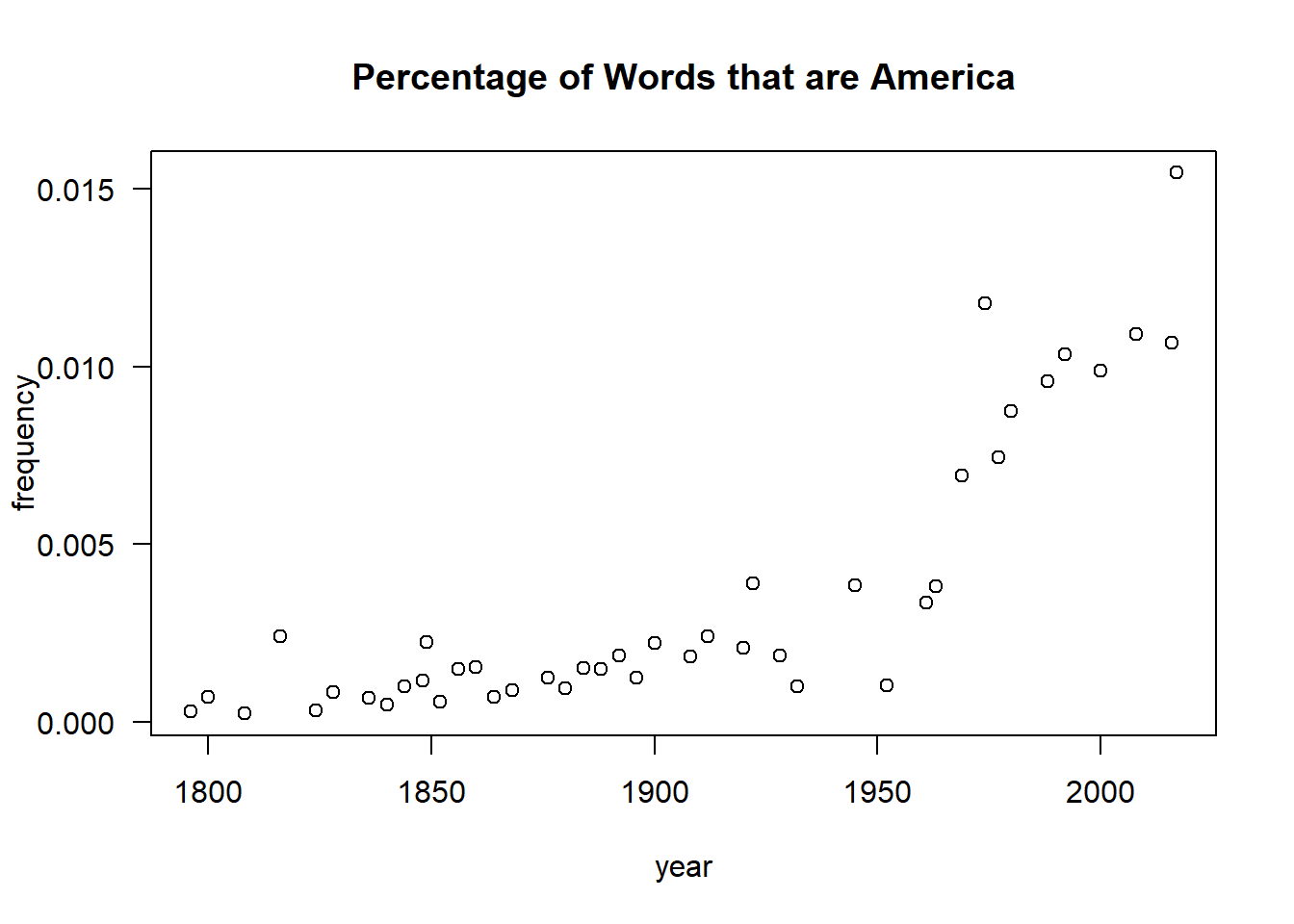
The following dataset comes from one I collected myself in 2016 by text mining the state of the union letters & addresses presented by the president of the Unites States since the founding of that country: The Frequency of America in America. This dataset counts the number of times each president says the word “America” or “American” in their State of the Union addresses. The dataset is as follows. Note that it ends in 2017 after Trump’s first State of the Union. This data was mined from https://www.presidency.ucsb.edu/.
# read in the datasotu =read.table("data/sotu.txt",header = T)head(sotu)
             indx AmerCnt  WCnt year
1 Washington    1       5 16587 1796
2 Adams         2       5  7149 1800
3 Jefferson     3       5 20576 1808
4 Madison       4      52 21622 1816
5 Monroe        5      14 42059 1824
6 Adams         6      26 30517 1828
tail(sotu)
           indx AmerCnt  WCnt year
40 Regan     40     345 35968 1988
41 Bush      41     181 17495 1992
42 Clinton   42     591 59858 2000
43 Bush      43     437 40029 2008
44 Obama     44     569 53346 2016
45 Trump     45      77  4984 2017
plot( sotu$year, sotu$AmerCnt/sotu$WCnt,xlab="year",ylab="frequency",las=1,main="Percentage of Words that are America")
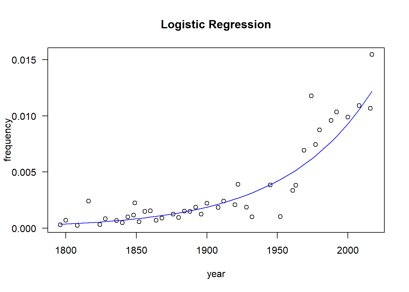
We can try to model these America counts as a binomial distribution with word count (WCnt) as the total number of trials. When we do a logistic regression like this, we use the weight argument to identify how many total trials occurred at each data point.
# Fit Logistic regression to frequenciesmd.logit =glm( (AmerCnt/WCnt)~year, data=sotu, weight=WCnt, family=binomial(link="logit") )summary(md.logit);
Call:
glm(formula = (AmerCnt/WCnt) ~ year, family = binomial(link = "logit"),
    data = sotu, weights = WCnt)

Coefficients:
              Estimate Std. Error z value Pr(>|z|)
(Intercept) -3.674e+01  5.052e-01  -72.71   <2e-16 ***
year         1.603e-02  2.586e-04   62.00   <2e-16 ***
---
Signif. codes:  0 '***' 0.001 '**' 0.01 '*' 0.05 '.' 0.1 ' ' 1

(Dispersion parameter for binomial family taken to be 1)

    Null deviance: 4761.11  on 42  degrees of freedom
Residual deviance:  542.39  on 41  degrees of freedom
  (2 observations deleted due to missingness)
AIC: 805.45

Number of Fisher Scoring iterations: 4
While there is no global test included in the GLM summary, we can test the overall fit of our logistic regression model using anova in R. However, this function allows us to choose our test statistic being one of “Chisq”, “LRT”, “Rao”, “F” or “Cp”. The LRT is our likelihood ratio test, which is standard to use in GLMs. Meanwhile, the F-test is said to be “inappropriate” as we are not independently estimating the mean and variance in this model.
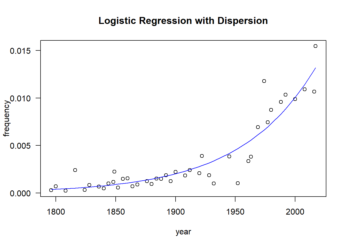
In the next lines of code, we switch from binomial to quasibinomial. This means that we are introducing a dispersion parameter, which allows for the variance to deviate from \(\pi(1-\pi)\). In this case, we have an under-dispersed logistic regression. Note that over-dispersion is typically more common in practice. Also, note that the hypothesis test distributions have changed from normal (z) to t. Furthermore, R is now okay with you using either the LRT or F test.
Call:
glm(formula = (AmerCnt/WCnt) ~ year, family = quasibinomial(link = "logit"),
    data = sotu)

Coefficients:
              Estimate Std. Error t value Pr(>|t|)
(Intercept) -36.748662   2.330116  -15.77   <2e-16 ***
year          0.016080   0.001187   13.54   <2e-16 ***
---
Signif. codes:  0 '***' 0.001 '**' 0.01 '*' 0.05 '.' 0.1 ' ' 1

(Dispersion parameter for quasibinomial family taken to be 0.0005740057)

    Null deviance: 0.154674  on 42  degrees of freedom
Residual deviance: 0.021324  on 41  degrees of freedom
  (2 observations deleted due to missingness)
AIC: NA

Number of Fisher Scoring iterations: 9
plot( sotu$year, sotu$AmerCnt/sotu$WCnt,xlab="year",ylab="frequency",las=1,main="Logistic Regression with Dispersion")lines( sotu$year[c(-9,-20)],1/(1+exp(-predict(md.logit))),col="blue" )
The estimated parameter for the year variable is 0.016, Which means that our fitted model looks like \[
\log \text{odds} = -36.75 + 0.016(\text{year})
\] Instead of a logistic regression, we can recall that a Binomial\((n,p)\) distribution with \(n\) large and \(p\) small is very close to a Poisson\((\lambda)\) distribution with \(\lambda=np\). Hence, we can try to model this same data using a Poisson regression with a log link function. This is another type of log linear model we are fitting.
# Fit Poisson regression to frequenciesmd.pois =glm( AmerCnt~year+WCnt, data=sotu, family=poisson(link="log") )summary(md.pois);
Call:
glm(formula = AmerCnt ~ year + WCnt, family = poisson(link = "log"),
    data = sotu)

Coefficients:
              Estimate Std. Error z value Pr(>|z|)
(Intercept) -2.648e+01  5.456e-01  -48.54   <2e-16 ***
year         1.580e-02  2.758e-04   57.31   <2e-16 ***
WCnt         1.590e-05  3.790e-07   41.94   <2e-16 ***
---
Signif. codes:  0 '***' 0.001 '**' 0.01 '*' 0.05 '.' 0.1 ' ' 1

(Dispersion parameter for poisson family taken to be 1)

    Null deviance: 5687.13  on 44  degrees of freedom
Residual deviance:  919.57  on 42  degrees of freedom
AIC: 1184.8

Number of Fisher Scoring iterations: 5
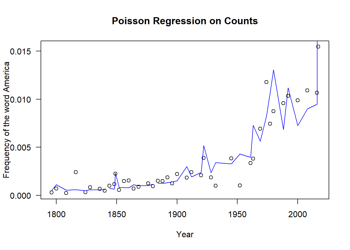
However, now we have an overdispersed Poisson regression, so we fit that model next. Note that the estimated parameters have not changed, but the test statistics and null distributions have. Albeit, they are all still significant.
# Plot raw countsplot( sotu$year,sotu$AmerCnt/sotu$WCnt,las=1,xlab="Year",ylab="Frequency of the word America",main="Poisson Regression on Counts")# Fit Poisson regression to frequenciesmd.pois =glm( AmerCnt~year+WCnt, data=sotu, family=quasipoisson(link="log") )summary(md.pois);
Call:
glm(formula = AmerCnt ~ year + WCnt, family = quasipoisson(link = "log"),
    data = sotu)

Coefficients:
              Estimate Std. Error t value Pr(>|t|)
(Intercept) -2.648e+01  2.469e+00 -10.727 1.32e-13 ***
year         1.580e-02  1.248e-03  12.666 6.20e-16 ***
WCnt         1.590e-05  1.715e-06   9.269 1.03e-11 ***
---
Signif. codes:  0 '***' 0.001 '**' 0.01 '*' 0.05 '.' 0.1 ' ' 1

(Dispersion parameter for quasipoisson family taken to be 20.47391)

    Null deviance: 5687.13  on 44  degrees of freedom
Residual deviance:  919.57  on 42  degrees of freedom
AIC: NA

Number of Fisher Scoring iterations: 5
The estimated parameter for the year variable is now 0.0158. Now the fitted model is \[
\log \text{counts} =
-26.48 + 0.0158(\text{year}) + 0.0000159(\text{words})
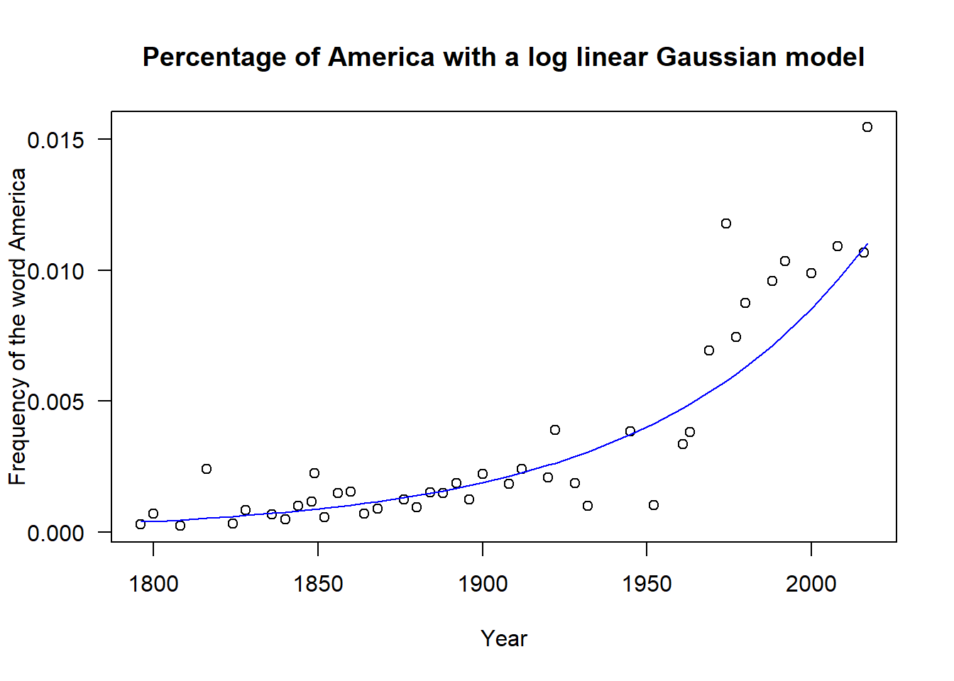
\] But we can go even further as the Poisson\((\lambda)\) distribution is approximately normal after properly scaling it for the central limit theorem. Hence, we can fit yet another log linear model using the normal distribution as we did in all the previous chapters of these notes.
# Fit log transformed linear modelmd.log =lm( log(AmerCnt/WCnt)~year, data=sotu,subset=-c(9,20) )summary(md.log);
Call:
lm(formula = log(AmerCnt/WCnt) ~ year, data = sotu, subset = -c(9,
    20))

Residuals:
     Min       1Q   Median       3Q      Max
-1.38176 -0.31175  0.02739  0.29912  1.49995

Coefficients:
              Estimate Std. Error t value Pr(>|t|)
(Intercept) -34.841650   2.319339  -15.02  < 2e-16 ***
year          0.015039   0.001218   12.35  2.1e-15 ***
---
Signif. codes:  0 '***' 0.001 '**' 0.01 '*' 0.05 '.' 0.1 ' ' 1

Residual standard error: 0.5097 on 41 degrees of freedom
Multiple R-squared:  0.7882,    Adjusted R-squared:  0.783
F-statistic: 152.6 on 1 and 41 DF,  p-value: 2.104e-15
# Plot log frequencies with a Gaussian modelplot( sotu$year,sotu$AmerCnt/sotu$WCnt,las=1,xlab="Year",ylab="Frequency of the word America",main="Percentage of America with a log linear Gaussian model")lines( sotu$year[c(-9,-20)],exp(predict(md.log)),col="blue" )
    DIV     time date    sex ageGroup      age
1 M3039 89.35000    1   male     3039 31.08459
2 M3039 90.18333    1   male     3039 37.77738
3 F5059 90.78333    1 female     5059 59.39656
4 M2029 90.90000    1   male     2029 22.49744
5 F3039 92.06667    1 female     3039 31.11756
6 M3039 93.23333    1   male     3039 36.22344
xx =sort( hypoDat$age )ord =order(hypoDat$age )
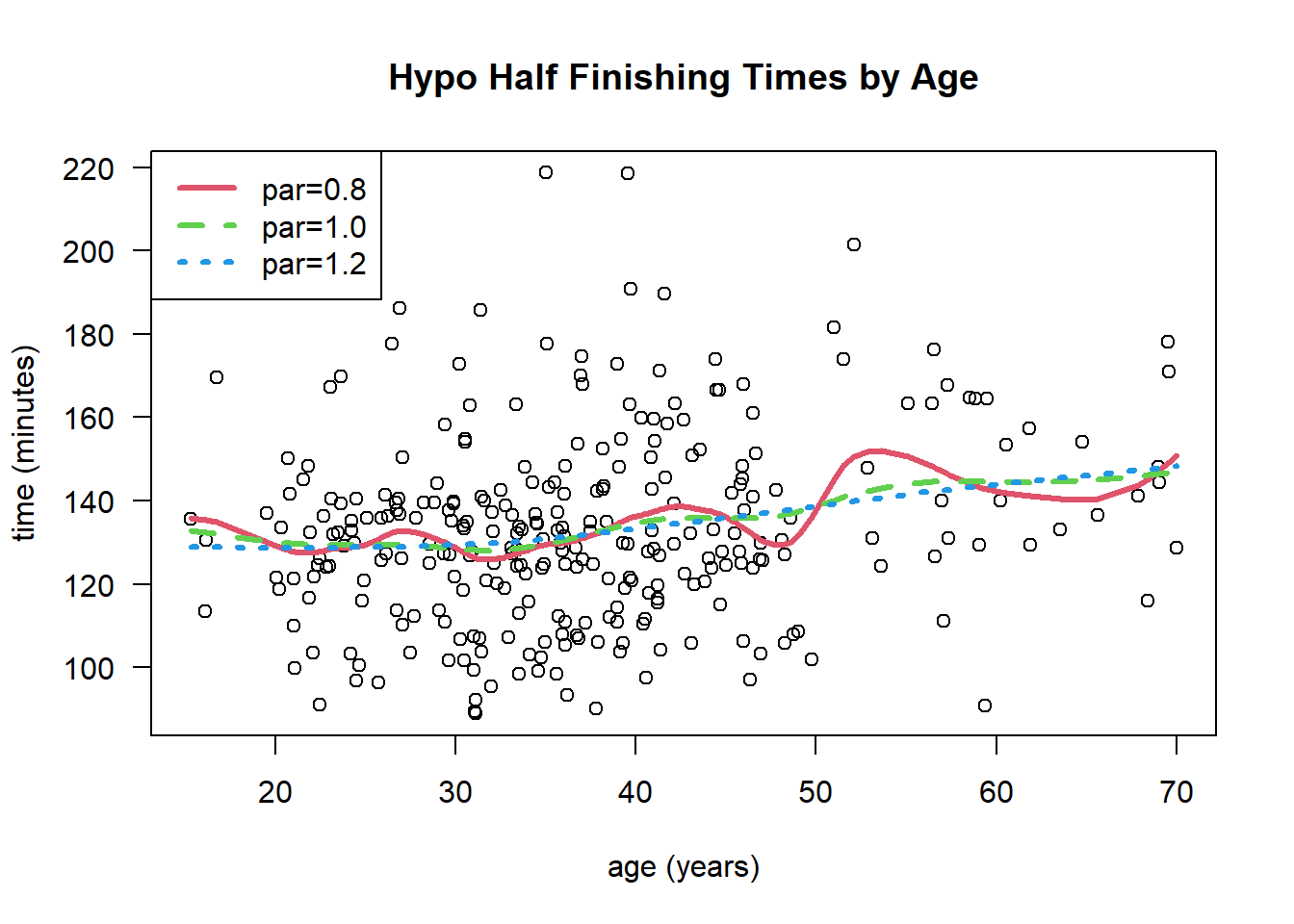
We can also use the R function smooth.spline() to fit a cubic smoothing spline to the data. The results are below where we vary the choice of smoothing parameter.
ss.a <-smooth.spline(x = xx, y = hypoDat$time[ord],spar=0.8)ss.b <-smooth.spline(x = xx, y = hypoDat$time[ord],spar=1.0)ss.c <-smooth.spline(x = xx, y = hypoDat$time[ord],spar=1.2)plot( hypoDat$age, hypoDat$time, las=1,ylab="time (minutes)",xlab="age (years)",main="Hypo Half Finishing Times by Age")lines( ss.a, lwd=3,lty=1,col=2 )lines( ss.b, lwd=3,lty=2,col=3 )lines( ss.c, lwd=3,lty=3,col=4 )legend("topleft",legend=c("par=0.8","par=1.0","par=1.2"),lwd=3,lty=1:3,col=2:4)